De-Novo Genome Assembly Containerized Pipelines
Welcome to your ultimate guide for using ready to go, containerized workflows for analyzing genome data.
So you have sampled your organism of interest, sequenced the data, and found yourself with a bunch of NGS reads that need to be analyzed. But, you don’t really know how to proceed, or, you do know, but you would rather spend your time writing your papers or examining other organisms in the meantime. In both cases, you are in the right place at the right time.
What you will find and what will you need to use it
The pipeline for genome assembly analyses is made using Snakemake and containerized through Singularity with the help of the Conda package manager. If you are not familiar with any of these tools, don’t worry. All you have to know, is that these technologies, give you the opportunity to transfer the workflow on any machine, as long as it works with a linux-based kernel and has Singularity installed. If these apply, you can run the pipeline effortlessly, without worrying about releases and packages that may not be compatible with each other. Conda handles that, and creates environments for the Snakemake workflow to run, without interferring with the system you are hosting it into.

The marriaging of these three tools, create the pipelines and deliver them to you in the form of container images. Each ready to use pipeline is represented by an image, and can be run in any cluster or environment that supports the resources and 3d parties tools needed.
In order for you to have some impact on the analysis and to also include your preferences in the procedure, the including and careful filling of a configuration file with lots of parameters is mandatory.
When it comes to genome analysis, you can choose out of four different images, depending on your needs and the data you have available. Here is a brief explanation for each one of them:
A. SQTQ
Short Quality-Trimming-Quality (SQTQ) is an image suitable for those who want to run a simple quality control for their short (Illumina) reads, before and after trimming them, when planning to use long and short reads combination for assembling a genome. It actually performs quality check on the raw data, trimming of the raw data and quality check all over again. The results of the image are the following, located in the same directory your raw data live in:
- One directory that contains the now trimmed short data, named trimmomatic_output
- One directory that contains the results of the quality control of the raw short reads, named Multiq_raw_report
- One directory that contains the results of the quality control of the trimmed short reads, named Multiq_trimmed_report
Here are the tools used for this analysis:
| Tools | Description | Version |
|---|---|---|
| fastqc | Quality check | 0.11.8 |
| Multiqc | Quality check | 1.6 |
| Trimmomatic | Trimming | 0.39 |
B. LQTQ
Long Quality-Trimming-Quality (LQTQ) is an image suitable for those who want to run a simple quality control for their long (MinION) reads, before and after trimming them. It actually performs quality check, trimming of the raw data and quality check all over again. The results of the image are again, the following three, located in the same directory your long, raw data live in:
- One fastq file that contains the now trimmed data, named porechop_output.fastq.gz
- One directory that contains the results of the quality control before trimming, named Nano_Raw_Report
- One directory that contains the results of the quality control after the trimming, named Nano_Trimmed_Report
Here are the tools used for this analysis:
| Tools | Description | Version |
|---|---|---|
| NanoPlot | Quality check | 1.29.0 |
| Porechop | Trimming | 0.2.3 |
C. LGA
Long Genome Assembly (LGA) is an image suitable for those who want to run a whole genome assembly analysis from start to end, and got only long (MinION) reads at their disposal. Here are the main tools used by the pipeline, and all the results the image is spawning:
LQTQ is part of LGA
- One fastq file that contains the now trimmed data, named porechop_output.fastq.gz
- One directory that contains the results of the quality control before trimming, named Nano_Raw_Report
- One directory that contains the results of the quality control after the trimming, named Nano_Trimmed_Report
- One directory called Assemblies, which will actually contain all the assemblies made through the procedure and polishing steps alongside the final assembly. It contains the following subfolders and files:
- (DIR) Flye: A folder containing the new assembly called assembly.fasta, and other side files.
- (DIR) Racon: A folder containing the (compressed) results and side files (s.a. .mmi files) for running Racon. These results, have a prefix or suffix (x), where (x) is a number and depends on the polishing rounds you’ve demanded in the configuration file. If for example your hyperparameter is 2, you will find four such files: 1_minimap.sam and 2_minimap.sam, racon_1.fasta, and racon_consensus.fasta. The last file is the final result of this part, has the string “consensus” rather than a number, and serves as input to Medaka.
- (DIR) (Lineage_name): A folder containing information about the lineage used for the BUSCO analysis below. (e.g.actinopterygii_odb9)
- (F) The .tar form of the above lineage folder.
- (DIR) Medaka: A folder containing the final, fully polished assembly called consensus.fasta, and other side files.
- One directory that contains the results of the BUSCO quality controls after each assembly creation, named Busco_Results. It contains two subfolders, QA_1 and QA_1, for assembly.fasta and for consensus.fasta respectively.
- One directory that contains the results of the QUAST quality controls after each assembly creation, named Quast_Results. It contains two subfolders, QA_1 and QA_2, for assembly.fasta and for consensus.fasta respectively.
- A pdf in the same directory with the image, with a directed acyclic graph (DAG) generated by it, which shows the dependencies and input-outputs of the jobs of the image for you to check and use as you like.
- A .txt file named “Summary.txt”, which contains information about the completeness of the files generated by the pipeline.
| Tools | Description | Version |
|---|---|---|
| NanoPlot | Quality check | 1.29.0 |
| Porechop | Trimming | 0.2.3 |
| Flye | Assembler | 2.6 |
| Busco | Quality check | 3.0 (Internal Blast: v2.2) |
| Quast | Quality check | 5.0.2 |
| Racon | Polishing | 1.4.12 |
| Medaka | Polishing | 0.9.2 |
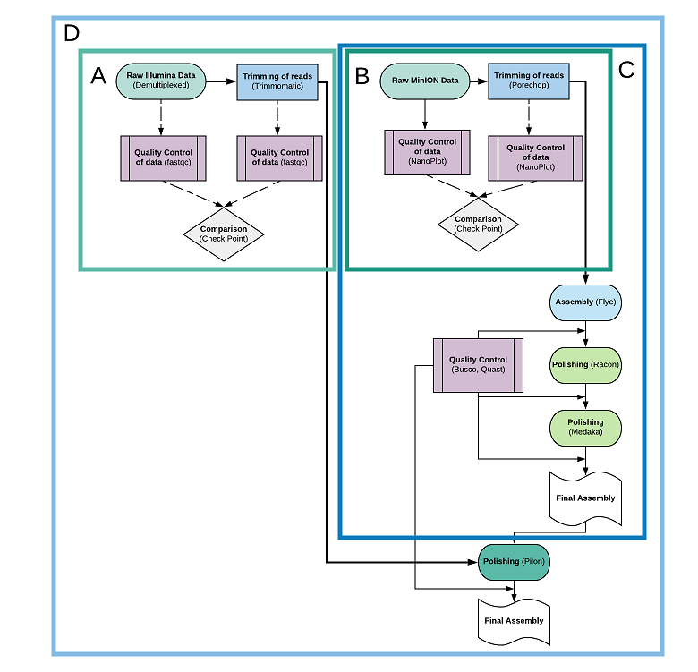
D. LSGA
Long-Short Genome Assembly (LSGA) is an image suitable for those who want to run a whole genome assembly analysis from start to end, and got both long (MinION) reads and short (Illumina) reads at their disposal. Here are the tools and all the results the image is spawning:
All the other images are part of LSGA.
- One directory that contains the now trimmed short data, named trimmomatic_output
- A directory called KmerGenie inside the trimmomatic_output dir, generated by the KmerGenie program and informing about the estimated genome size for the assembly and the kmers of the data, used later as parameter for the Flye Assembler.
- One directory that contains the results of the quality control before trimming the short reads, named Multiq_raw_report
- One directory that contains the results of the quality control after trimming the short reads, named Multiq_trimmed_report
- One fastq file that contains the now trimmed data, named porechop_output.fastq.gz
- One directory that contains the results of the quality control before trimming, named Nano_Raw_Report
- One directory that contains the results of the quality control after the trimming, named Nano_Trimmed_Report
- One directory called Assemblies, which will actually contain all the assemblies made through the procedure and polishing steps alongside the final assembly. It contains the following subfolders and files:
- (DIR) Flye: A folder containing the new assembly called assembly.fasta, and other side files.
- (DIR) Racon: A folder containing the (compressed) results and side files (s.a. .mmi files) for running Racon. These results, have a prefix or suffix (x), where (x) is a number and depends on the polishing rounds you’ve demanded in the configuration file. If for example your hyperparameter is 2, you will find four such files: 1_minimap.sam and 2_minimap.sam, racon_1.fasta, and racon_consensus.fasta. The last file is the final result of this part, has the string “consensus” rather than a number, and serves as input to Medaka.
- (DIR) (Lineage_name): A folder containing information about the lineage used for the BUSCO analysis below. (e.g.actinopterygii_odb9)
- (F) The .tar form of the above lineage folder.
- (DIR) Medaka: A folder containing the final, fully polished assembly called consensus.fasta, and other side files.
- (DIR) One directory called Pilon_Results, which contains all the Pilon results, also with an iteration prefix. The number of iterations is decided based on whether the polishing rounds are advancing the quality of the assembly or not. Specifically, a quality control (BUSCO and QUAST) is made after each polishing round. If the “Missing BUSCOs” are at least 5 lesser than the previous round, and the Quast’s N50 is lowering by at least 500.000bp, the polishing is continued. If these conditions are not fulfilled anymore, the polishing is terminated. The final, fully polished assembly given to the user, is called final.fasta and can be found in this directory.
- One directory that contains the results of the BUSCO quality controls after each assembly creation, named Busco_Results. It contains two standard subfolders, QA_1 and QA_2, for assembly.fasta and for consensus.fasta respectively, and one more for each Pilon round, whith a suffix for the respected iteration.
- One directory that contains the results of the QUAST quality controls after each assembly creation, named Quast_Results. It contains two standard subfolders, QA_1 and QA_2, for assembly.fasta and for consensus.fasta respectively, and one more for each Pilon round, whith a suffix for the respected iteration.
- A pdf in the same directory with the image, with a directed acyclic graph (DAG) generated by it, which show the dependencies and input-outputs of the jobs of the image for you to check and use as you like.
- A .txt file named “Summary.txt”, which contains information about the completeness of the files generated by the pipeline.
| Tools | Description | Version |
|---|---|---|
| fastqc | Quality check | 0.11.8 |
| Trimmomatic | Trimming | 0.39 |
| Multiqc | Quality check | 1.6 |
| NanoPlot | Quality check | 1.29.0 |
| Porechop | Trimming | 0.2.3 |
| Flye | Assembler | 2.6 (Internal: KmerGenie: v1.70.16) |
| Busco | Quality check | 3.0 (Internal Blast: v2.2) |
| Quast | Quality check | 5.0.2 |
| Racon | Polishing | 1.4.12 |
| Medaka | Polishing | 0.9.2 |
| Pilon | Polishing | 1.23 (Internal: Samtools: v1.9, Minimap2: v2.17) |
Thus, in order for you to run your analysis in your organism’s or industry’s server, all you need is:
- A server that has Singularity installed
- The image of the pipeline you wish to use for your analysis
- The corresponding configuration file along with the image, that lets you define different parameters for the analysis
- A script that submits the image as a job into the nodes of your cluster
Breaking down the steps that lead to the analysis
Having found the image that correspond to the analysis you need, download it and copy it along with the configuration file in the home folder of your cluster account. A simple cp or a scp will do the trick. Once you’re done, open the configuration file with nano to edit it. The configuration file is probably the most important component for your analysis to work, so take your time and double check all the paths and the parameters needed here. The file is made to work for all the currently available analyses, so your intervention and filling will in fact let the whole system know which image you are going to use and thus the goal of your chosen pipeline, so make sure to fill the right variables in order for your image to be executed properly. Inside the configuration file you will also find some requirements that your raw data should fulfill. If your data or data directories do not follow the standards, please make the appropriate changes before editing the configurations. The cleaness of your directories is also very important. The workflow generates many intermediate files while running, and deletes them when not using them anymore, in order for your outputs to be carefully and tidy arranged, and your account free of unnecessary files. In order for the workflow to not mistakenly read or delete a file with the same name or regular expression of the file it is truly looking for, the directory where you copy the image and the configuration file into should be empty, and the directories of your raw data should not contain anything more or less than the data itself. Clean the necessary directories before filling the configuration file, to avoid any mistakes. If you wish to re-run the workflow for any reason (errors or verifications), make sure to delete or move any already created output before proceeding.
Once done with all that, it’s time to let the automated workflow do the rest for you. Follow the standars for running a job on your server’s cluster and submit the image as follows (replacewith the name of the actual image you have chosen, and add any path needed): singularity run <image.simg>When the workflow is done, check carefully if all the files that should have been spawned are present in your directories, as and their status in the Summary.txt file. Ignore any other file mentioned, that may be spawned intermediately and has already been deleted by the workflow a priori.
Note: The LGA and (especially) LSGA pipelines spawn a lot of files and data. Bare in mind that you should have enough space before running them in your repositories. The needed space varies, because the round of for example the Pilon rounds are not predetermined, and thus the number of outputs is not known a priori. The optimity is accomplished when running with cpus multiples of ten (10,20,30 etc.).
Pipelines:
If you wish to use our images, get in contact with us for the necessary files.
Developers:
If you are a developer and you wish to explore our code and learn more about these technologies, ask for access to our GitHub repository for developers and maintainers.
Credits and Citations:
- Köster, Johannes and Rahmann, Sven. “Snakemake - A scalable bioinformatics workflow engine”. Bioinformatics 2012.
- Kurtzer GM, Sochat V, Bauer MW (2017), Singularity: Scientific containers for mobility of compute. PLoS ONE 12(5): e0177459.
- Crist-Harif et al, Conda, GitHub repository: https://github.com/conda.
- Andrews S. (2010). FastQC: a quality control tool for high throughput sequence data. Available online at: http://www.bioinformatics.babraham.ac.uk/projects/fastqc.
- Bolger, A. M., Lohse, M., & Usadel, B. (2014). Trimmomatic: A flexible trimmer for Illumina Sequence Data. Bioinformatics, btu170.
- Philip Ewels, Måns Magnusson, Sverker Lundin, Max Käller, MultiQC: summarize analysis results for multiple tools and samples in a single report, Bioinformatics, Volume 32, Issue 19, 1 October 2016, Pages 3047–3048.
- Wouter De Coster, Svenn D’Hert, Darrin T Schultz, Marc Cruts, Christine Van Broeckhoven, NanoPack: visualizing and processing long-read sequencing data, Bioinformatics, Volume 34, Issue 15, 01 August 2018, Pages 2666–2669.
- R. Wick, Porechop (2017), GitHub Repo: P.W.D. Charles, Project Title, (2013), GitHub repository: https://github.com/rrwick/Porechop.
- Kolmogorov, M., Yuan, J., Lin, Y. et al. Assembly of long, error-prone reads using repeat graphs. Nat Biotechnol 37, 540–546 (2019).
- Heng Li, Minimap2: pairwise alignment for nucleotide sequences, Bioinformatics, Volume 34, Issue 18, 15 September 2018, Pages 3094–3100.
- Li H, Handsaker B, Wysoker A, et al. The Sequence Alignment/Map format and SAMtools. Bioinformatics. 2009;25(16):2078‐2079.
- Vaser R, Sović I, Nagarajan N, Šikić M. Fast and accurate de novo genome assembly from long uncorrected reads. Genome Res. 2017;27(5):737‐746.
- Oxford Nanopore Technologies, Medaka 2018, GitHub repository: https://github.com/nanoporetech/medaka
- Bruce J. Walker, Thomas Abeel, Terrance Shea, Margaret Priest, Amr Abouelliel, Sharadha Sakthikumar, Christina A. Cuomo, Qiandong Zeng, Jennifer Wortman, Sarah K. Young, Ashlee M. Earl (2014) Pilon: An Integrated Tool for Comprehensive Microbial Variant Detection and Genome Assembly Improvement. PLoS ONE 9(11): e112963.
- Gurevich A, Saveliev V, Vyahhi N, Tesler G. QUAST: quality assessment tool for genome assemblies. Bioinformatics. 2013;29(8):1072‐1075.
- Felipe A. Simão, Robert M. Waterhouse, Panagiotis Ioannidis, Evgenia V. Kriventseva, Evgeny M. Zdobnov, BUSCO: assessing genome assembly and annotation completeness with single-copy orthologs, Bioinformatics, Volume 31, Issue 19, 1 October 2015, Pages 3210–3212.
- Rayan Chikhi, Paul Medvedev, Informed and automated k-mer size selection for genome assembly, Bioinformatics, Volume 30, Issue 1, 1 January 2014, Pages 31–37.
Please credit accordingly:
Author: Nellie Angelova, Bioinformatician, Hellenic Centre for Marine Research (HCMR)
Coordinator/ Supervisor: Tereza Manousaki, Researcher, Hellenic Centre for Marine Research (HCMR)
Contact: n.angelova@hcmr.gr